Before adding risks to the pool and add funding coverage against them, there are a number of decisions or areas of understanding and prioritisation that have to be established outside of the tool and the calculation.
What risks should be covered financially and include in the pool?
The risks to cover will likely be different for all organisations and will be dependent on several factors. This may be depend on the risks and impacts that a country has prioritised. It may include looking at the operational systems that are ready to utilise the money effectively in emergencies. How those country risks are identified will require decision-making criteria on those being prioritised for coverage.
Who has requested coverage and how much?
Firstly, there is likely to be a mechanism where those who would be utilising the pre-positioned disaster funding could request coverage support. Certain conditions may be in place for prepositioned funding coverage. These may be how effective and well-planned the delivery of support with the released funding is or potentially what existing financial coverage and support is already in place. How to consider those requests will depend on existing governance and requirements, which should be clarified for transparency.
What type of coverage has been requested?
How much funding has been requested for different levels of risk needs to be considered in the financial structure. There may be preferences for more funding for different severity events, depending on the financial needs and gaps.
What other funding coverage is in place for those risks?
Providing funding coverage from the pool for the entirety of the possible funding risk is unlikely. Often, a mixture of funding lines come in for different emergencies and at different severities. So, understanding the landscape in which the pool sits will be important before constructing the financial structuring. This will ensure the most efficient arrangement of funding for future crises is used. Having pre-arranged financing for a crisis also means that the corresponding emergency planning and operations will be incentivised to do the same. Chaotic financing systems often intersect in creating chaotic operational systems in disasters.
The first step is gathering data on past events for the risks to be included in the pool. This includes the perils and which countries were affected, in addition to impact metrics such as people affected or financial costs.
1. Identify which risks to include in the risk pool:
A ‘risk’ refers to a combination of hazard and country historical data.
Risks included in a risk pool are contractually covered by the risk pool and would receive guaranteed pay-outs upto a pre-agreed amount, if a loss was to occur for that hazard and country combination in the future.
2. Build or locate a historical event catalog containing:
Year of Event
Country
Peril (Hazard)
Loss Amount (for this tool, convert any financial losses (or response cost to USD)
Data sources could include public loss databases (e.g., EM-DAT), records from local stakeholders, and in-house or external models. Working with local agencies and stakeholders to identify and validate past data on events is key.
The Loss Simulator tool includes EM-DAT data historical loss by default. The tool allows you to select a country and run that historical data through the simulation engine to prepare losses for use in the Disaster Risk Pool Structuring Tool (see Phase 2 Step 3 for more).
3. Identify possible sources of error:
Gaps in historical records, i.e., missing events or years of observation
Use of different currency, and a need to scale for inflation, or misreporting of event information
Missing data (for example for smaller events - their impacts are less likely to be recorded in a global historical loss data catalogue)
What data is good enough to include in our catalogue?
“Good enough” is a relatively subjective term, so it will be important to have criteria in which past disaster data is deemed of sufficient quality to be included in your catalogue. In some cases, larger events and hazards, such as earthquakes and cyclones, which have clearer infrastructural-based impacts, may be easier to cross-reference and verify and therefore have more confidence in the loss data. Events like droughts and food security impacts can be more difficult to understand and definitively quantify. There should be clear rationale on why different types and sources of data have been included or excluded from the catalogue. It is important that the depiction of risk is kept as true as possible, without augmentation to a preferred view of risk for financial considerations. This should be done later on within the financial structuring.
What are the key instances and likely sources of error and uncertainty in the event data?
Knowing what gaps and limitations exist within your base event catalogue will give you indications for each risk when the risk relationship depicted may be over or underestimating the risk due to those limitations. The likely reasons for this are essential to note and identify to help with the later management of uncertainties and basis risk operationally.
Fundamental Principle
Magnitude refers to how big the event is - (this may be defined by the physical hazards, or the impact and losses - which are not the same), so make sure you know what kind of magnitude the data is showing you.
Frequency is how often that size magnitude event occurs. High magnitude events happen infrequently and low magnitude events happen more frequently. But the relationship between these variables will be different for each risk, location and circumstances. Understanding that relationship is the fundamental core to strategic risk management.
Climate Change doesn’t impact the day to day occurrences of events, but it does alter this magnitude frequency relationship over the long term.
Now you have a database of past event information on the risks that the pool will cover. This will provide information about the magnitude and frequency of those events and the overall likely financial need in total those types of crises may require. However, it will likely need some improvements using statistical techniques.
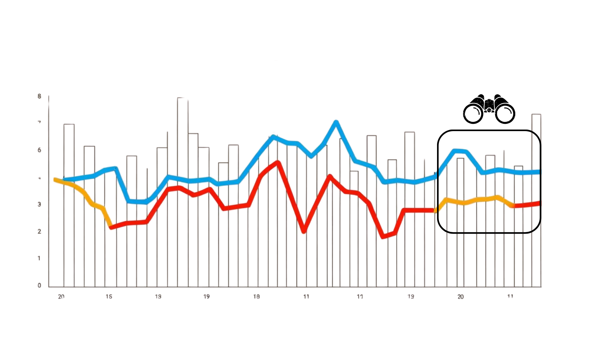
This is because, often, we will only have a small snapshot of those relationships and patterns, so we need ways to try to understand the broader relationship beyond the data we have for recorded events. The original dataset likely won’t cover all potential events of interest (i.e. even rare ones that may occur once every 200 years) and therefore statistical techniques are used instead to re[resent what we can’t see with our limited view.
Limited duration of event observation (boxed), and extension of that via stochastic simulation.
Step 2: Creating a Synthetic (Simulated) Loss Catalogue
This step shows how to use that information and to project, and better understand, the statistical patterns and likely probabilities of different events.
The Loss Simulator creates a set of synthetic (or simulated) event losses, based on historical loss data.
It is often difficult to understand long-term patterns of disaster impacts and losses because we typically have a short duration of recorded past event data. In some cases, there might only have two or three events with reliable data on impacts and losses. To address this, it is typical to create a stochastic set of events to model their impacts, or to statistically simulate a catalogue of losses. A relatively small number of events in a historical catalogue can be used to simulate tens of thousands of event losses, representing wider variability than shown in the historical record, and extreme losses that have not been captured in the historical record.
Fundamental Principle
How reliable is our understanding of the magnitude frequency patterns?
Reviewing the quality of the event data available and the robustness of the distribution fitting will give decision-makers a clear idea of how reliable our knowledge of the magnitude frequency relationship is. This is important as the weight of the risk in the pool may be under or overestimated due to this. When it comes later on to assigning financial coverage to those risks, this would need to be a consideration alongside the nature of the risk depicted in the distribution.
The Loss Simulator can be run in Basic Mode or Advanced Mode. It is recommended to begin with Basic Mode.
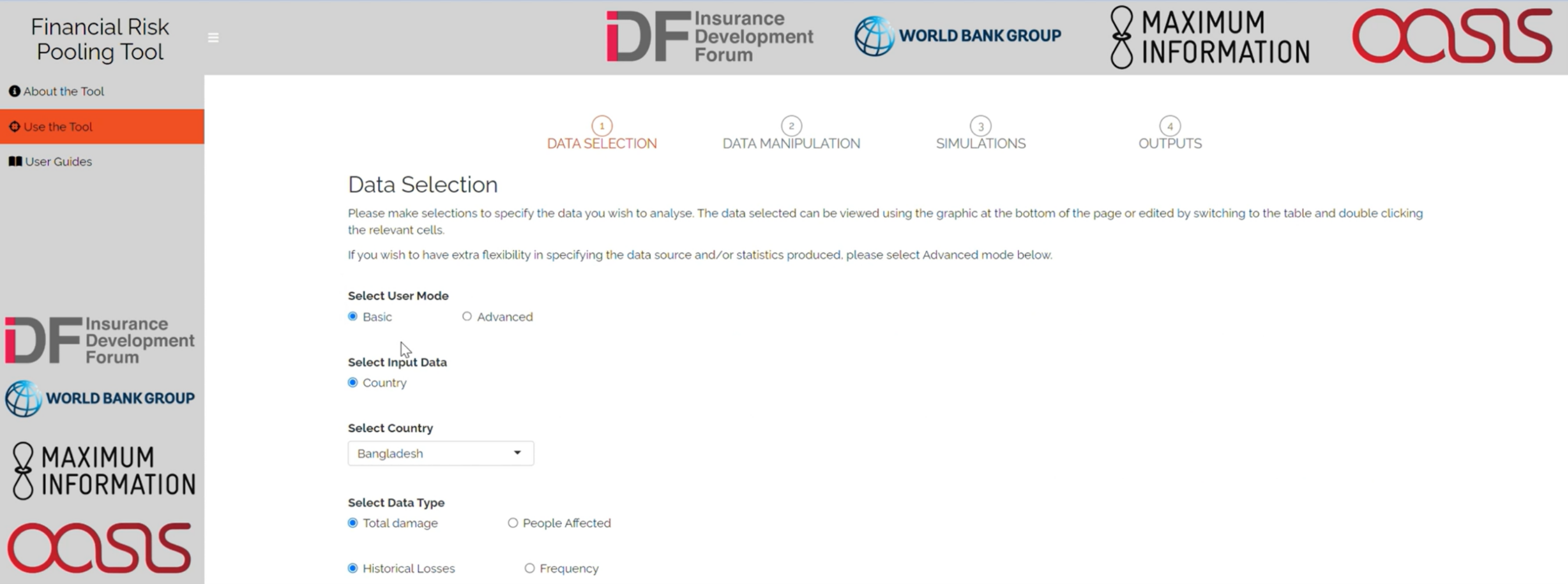
Data Selection Tab (Basic Mode)
This mode uses country input data pre-loaded into the Loss Simulator, from the EM-DAT global historical loss data catalogue
Select your country of analysis.
Select the impact metric you wish to use in the loss simulation. Your selection here determines the metric shown in the outputs and download for use in investigating the risk pool structure.
If using the simulated losses in a risk pool structure, use the same impact metric for all countries.
If ‘People Affected Response Cost’ is selected, there is an option to set the response cost per person. This value converts the number of people affected per event in EM-DAT, to a response cost per event. A response cost can be estimated using the average loss per person in the historical data where both are available, or there may be an otherwise established / estimated cost per person for the country.
The chart / table shows the annual response cost or economic damage per peril for the selected country, as given in EM-DAT. The frequency of events can also be shown. Events are shown on the chart only if the impact metric is non-zero in the historical loss catalogue. It is common for events to have a zero loss for Economic Damage and non-zero loss for people affected - therefore the number of events displayed will differ by impact metric selected. The metric type shown on this chart when you navigate to the next step (click ‘Next’), will be the metric used in the rest of the analysis.
The more historical event data you have from historical catalogs, the more robust the simulations will be to give the view of risk and the magnitude/frequency relationship. If only a small number of historical event information data points are available, there will be significant uncertainty in your financial risk modelling. This uncertainty increases if events close to your later attachment/trigger points are not well represented. Exercise caution in these cases as it may not be sensible to include risks based on such small amounts of data in the pool because they may not capture the potential funding liabilities.
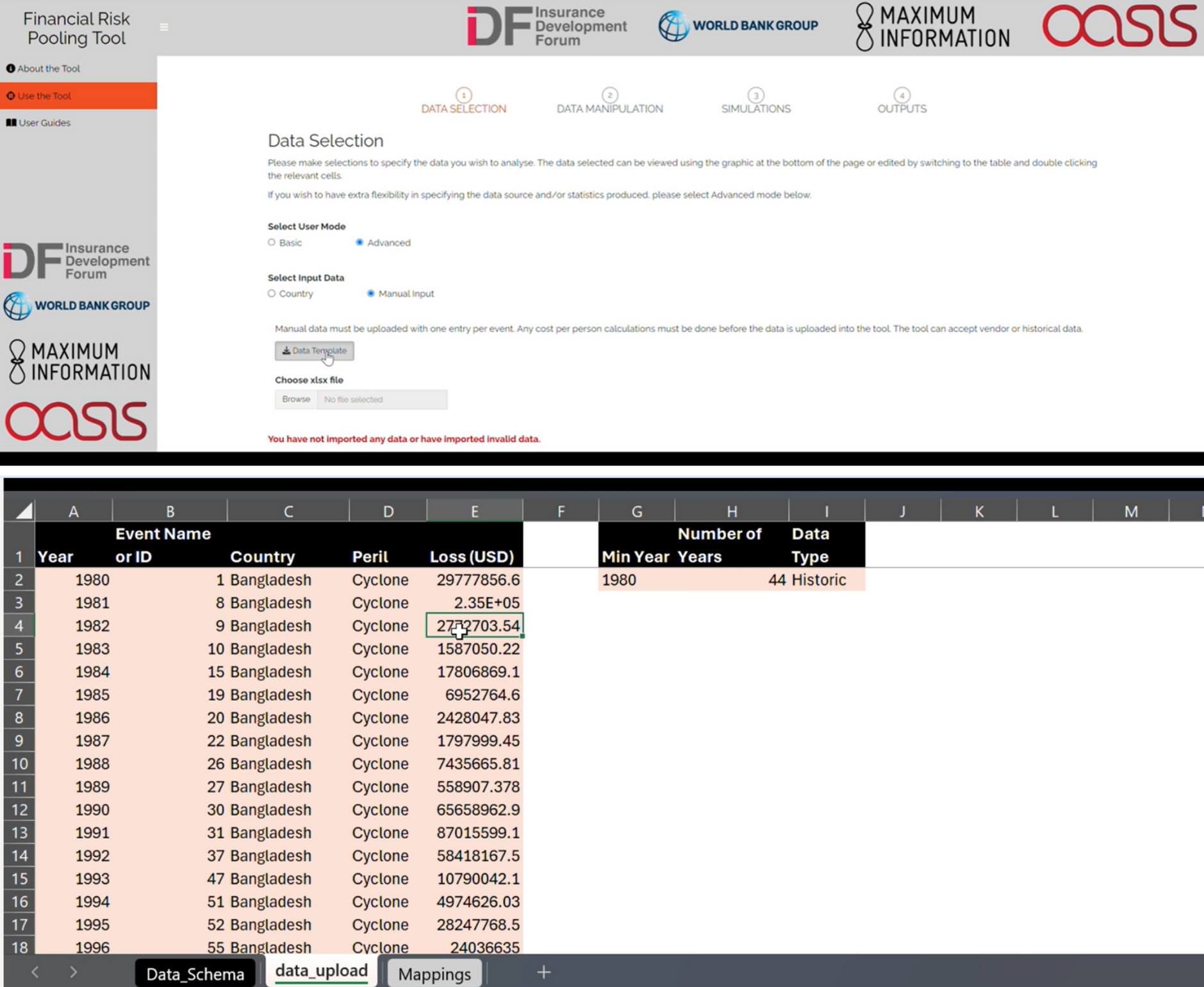
Data Selection Tab (Advanced mode): users choosing to use a different data source than provided in Basic Mode can upload their own event loss data using the Excel template provided along with a manual upload option, when Advanced Mode is selected. A graph of uploaded data appears at the bottom for validation, in the same way as it does on Basic Mode.
Advanced Mode offering data upload - also showing the manual input file format
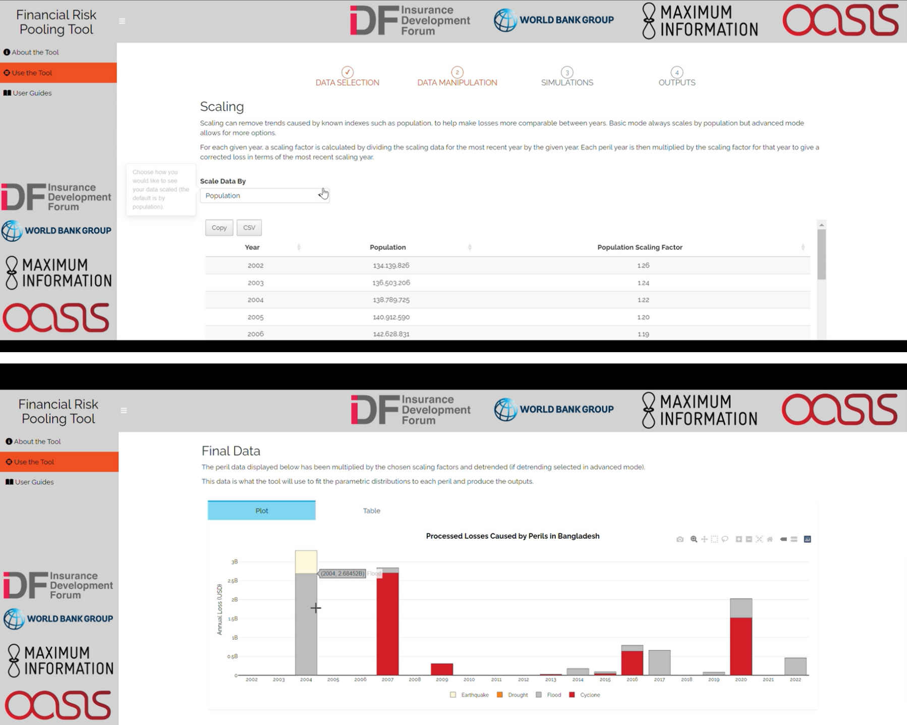
Scaling (Basic Mode)
The historical data can be scaled to reflect the impact of changing socio-economic conditions. In Basic Model the default is that the data is scaled by Popoulation using data pre-loaded in the Loss Simulator. This provides a scaling factor per year, which is applied to the original historical loss data.
The plot of ‘Final Data’ shows the scaled loss data.
In advanced mode there are more options to scale data by inflation or GDP, or use no scaling. Manual input data must attribute each loss to a specific year for scaling to be applied. If input data are scaled prior to input into the Loss Simulator., select ‘no scaling’ here.
Simulation
Click Run Tool to simulate event losses from the historical data. This could take up to 5 minutes).
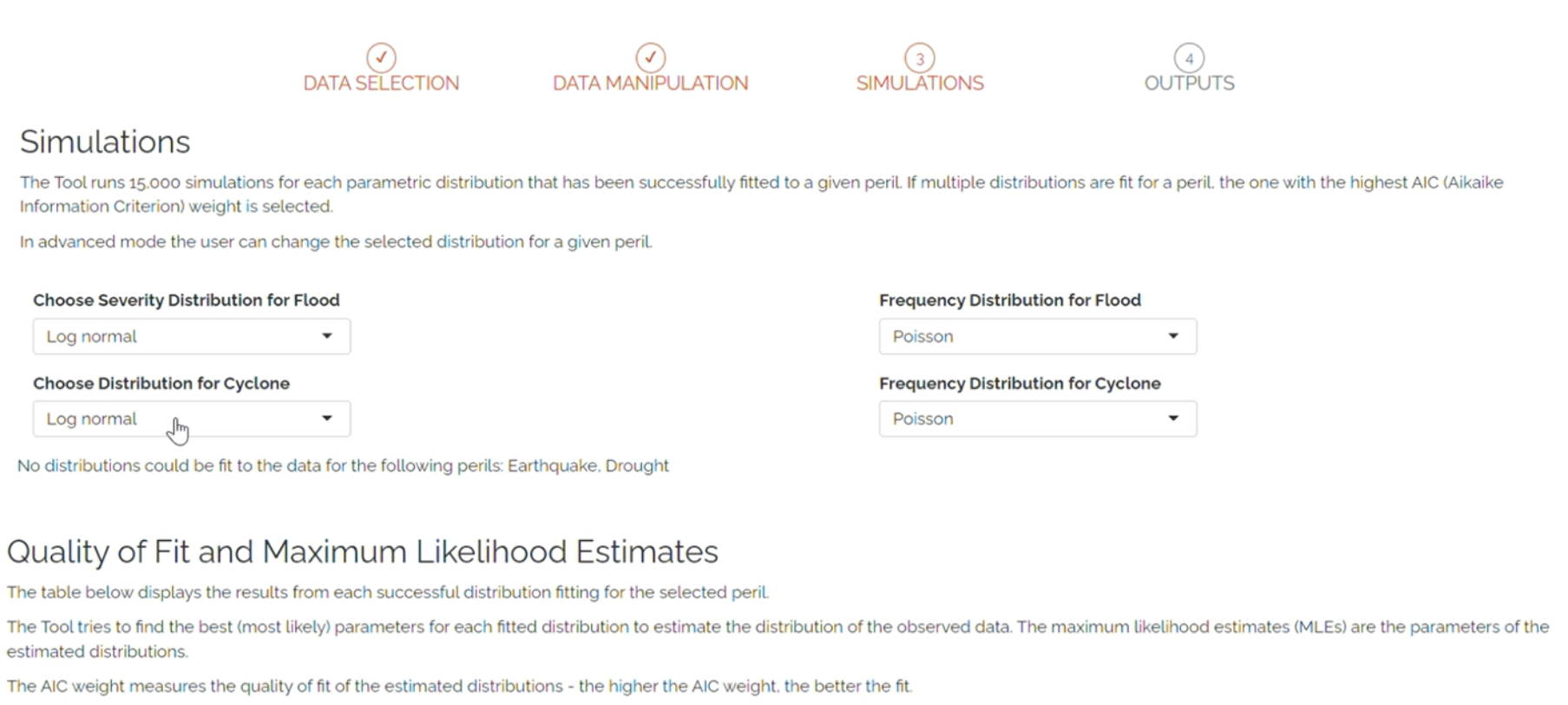
In both Basic mode and Advanced mode the tool fits multiple statistical distributions for loss amount (severity) and selects the distribution with the best possible fit to the data. The severity distributions tested by default are Lognormal, Gamma and Weibull.
In Advanced mode you can change the distribution selection - but it is advised to only do this with expert support.
For frequency of losses the tool tests the Poisson distribution assumption that sample variance equals the mean. If this is true in the data, Poisson frequency is used but where variance is less than the mean then the Negative Binomial frequency distribution is used.
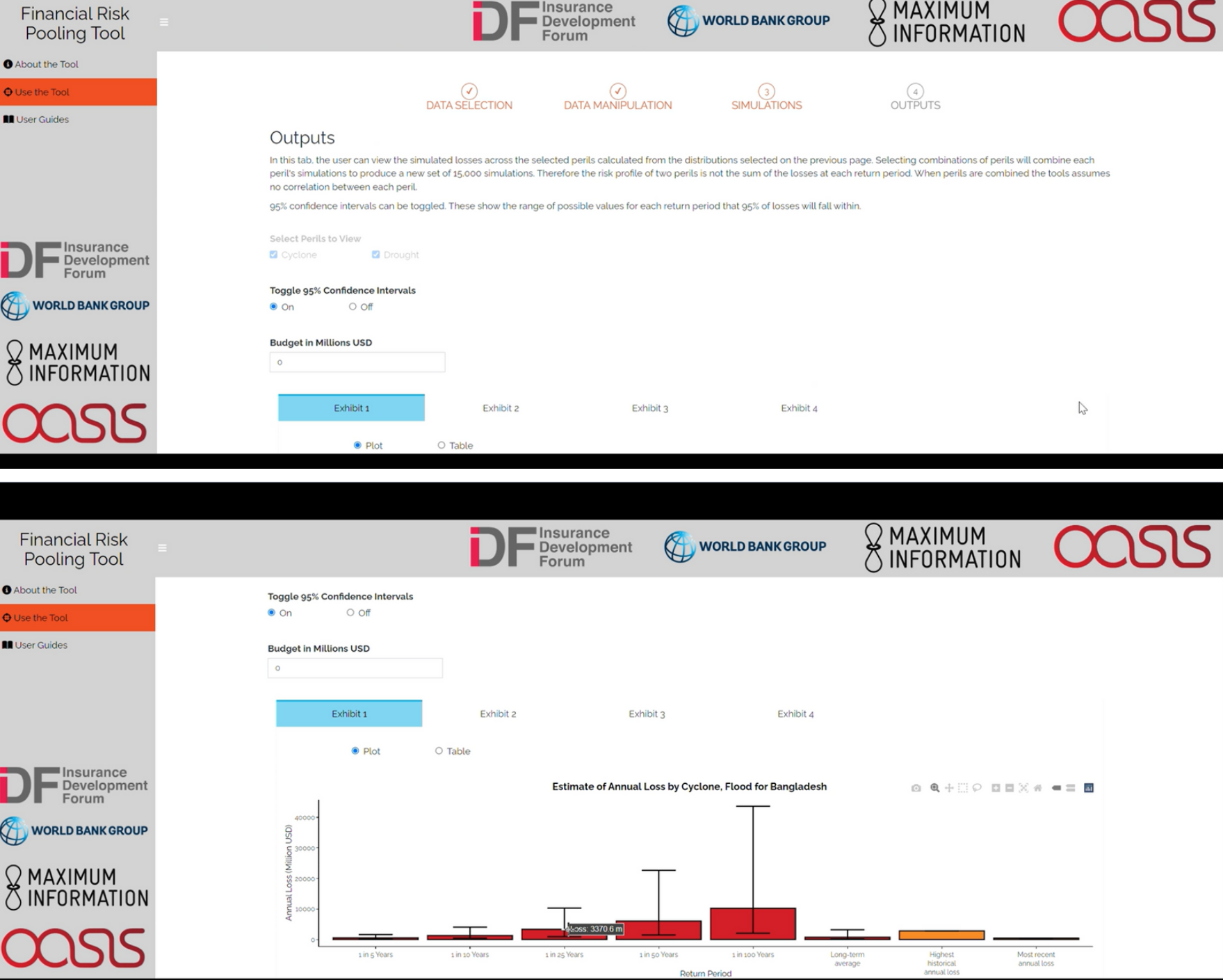
The ‘Outputs’ tab provides four exhibits from which to understand the simulated losses. Each exhibit provides a plot and a table of data.
Options:
Select which of the perils to view in the outputs.
Toggle 95% confidence intervals to see the range of uncertainty at each return period.
Enter a budget amount to compare losses to a budget.
The exhibits show:
Estimated annual losses for the country and peril(s) from the historical catalogue and the simulations. Return Period loss estimates are also shown from the simulated losses.
The Loss Exceedance curve from the simulated losses, with probability of exceeding the defined budget.
Average annual loss by likelihood - by defining a probability threshold for a ‘severe’ and ‘extreme’ loss, users can estimate what that level of loss looks like in terms of monetary amount.
Estimate of annual funding gap, based on comparison of the simulated loss severity and frequency, and the defined budget.
Download Simulations to save your new synthetic event catalog in the format needed for input into the Risk Pool Structuring tool. The data in this .csv file will need to be copied into the ‘Country Input’ sheets of the Risk Pool Structuring Tool.
Simulation outputs tab. Guidance on each exhibit is provided below the plot.
Now you have a database of observed and simulated crisis events and their losses, from which the patterns of magnitude and severity can be better understood.
Limitations: The Loss Simulator runs only type of input at a time. For example you cannot combine historical events _and_ modelled events for earthquake for a country. There is no consideration or estimation of correlation of losses between countries or perils in the Disaster Risk Pooling tool.**
In the next phase, you will use the Risk Pool Structuring tool to explore the principles of structuring a risk pool.
How many simulated events are enough?
How many simulations you include will depend on the computing power you have and also the number of events you are basing that simulation on. If like in the example, you only have 3 events with data. Running 20,000 events is likely going to be highly uncertain, so perhaps less is more in that case. A statistician or actuary would help you make a sensible choice.
What scaling to apply?
Here, it will consider what other changes happened alongside this data, which might influence the data and the objectivity of that pattern you are trying to understand. This can include population changes, price and cost changes with inflation. Once those trends are identified, the data related to them can be included to have those associated patterns in the data removed.
What statistical distributions will be used to generate the synthetic catalogue?
There are many different shapes of curves that can be plotted through the graph of the catalogue to try and discern most accurately the related pattern of magnitude and frequency of that risk. A statistician will look at different options to fit a curve. Usually, there will be no one perfect obvious pattern, so there will be trade-offs on which distribution is selected. Understanding the implications of those trade-offs in that decision would need to be understood by decision-makers where there may be over or under-estimates at different parts of the risk relationship.
What level of statistical uncertainty do we have?
How well the selected distribution fits the data will generate uncertainty, where the best fit is made. Statisticians will look to minimise the uncertainty as much as possible, but as with all things, this can only be minimised. Decision-makers will need to know, understand, and accept this.